
This has been my mantra for the past week. It seems as though there is always more to do, and I am finding myself perpetually exhausted…but I do not want to stop and even if I wanted to I can’t. Continue reading

This has been my mantra for the past week. It seems as though there is always more to do, and I am finding myself perpetually exhausted…but I do not want to stop and even if I wanted to I can’t. Continue reading
Another Saturday Skype call with T. Olga — my off-campus mentor who guides me through the sometimes-overwhelming world of academic literature — yielded one clear message: even more so than last week, I need to narrow my focus in order to not drown in sources turn out a paper by the end of May.

Usually, I begin my independent project with a blog post containing a detailed plan for the semester. This time, I feel compelled to write about an interesting experience with submitting my app to Apple’s App Store and getting it rejected twice by the App Review Board.

These are just some examples of things I have heard girls say to other girls or about other girls…within the past week. Continue reading
For my demonstration of learning last semester, I produced a review of literature pertaining to several important topics within Richard II’s reign (an overview of which can be found here) in the period between 1389-97. This period is not arbitrarily defined, but is marked by the two crisis which form its boundaries. Continue reading
The way in which people interact always fascinated me. Of course, during my early adolescence, I was just as confused as the next girl as to why my friends acted so mean at school. Beginning as early as second grade, our class was populated with cliques of girls who paraded around at recess and yelled at others for sitting on their slide, or wearing the same sparkly shirt as they did. Even at such a young age, the issue of girls fighting for power and social status was prevalent, and I wanted to know exactly why. Continue reading

Mass media and American foreign policy…. how does one even begin to narrow the focus of a project that considers a relationship of this magnitude?
Well, let’s start with what’s certain. I know that I want to write a paper. I also know that my independent is happening under the auspices of the history department, so a significant part of my paper would probably need to be devoted to combing through the history of America’s relationship with . . . which country? Never mind that, which region?

WEST CHESTER, Pennsylvania — January 20, 2018 — Today, Kevin Wang, designer of Westtown Resort and Polaris, announced Argus, an innovative iOS application that uses machine learning to perform scene and object recognition and enunciates what it detects to the user.

Tensorflow is one of the most widely used programming frameworks for algorithms with a large number of mathematical operations and computations. Specifically, Tensorflow is designed for the algorithms of Machine Learning. Tensorflow was first developed by Google and its source code soon became available on Github, the largest open-source code sharing website. Google uses this library in almost its all Machine Learning applications. From Google photos to Google Voice, we have all been using Tensorflow directly or indirectly, while a fast-growing group of independent developers incorporates Tensorflow into their own software. Tensorflow is able to run on large clusters of computing hardware and its excellence in perceptual tasks gives it an edge to Tensorflow in competitions against other Machine Learning libraries.
In this blog, we will explore the conceptual structure of Tensorflow. Although Tensorflow is mostly used along with the programming language Python, only fundamental knowledge of computer science is needed for you to proceed further in this blog. As its name suggests, Tensorflow comprises two core components: the Tensors and the computational graph (or “the flow”). Let me briefly introduce each of them.
Mathematically speaking, a Tensor is an N-Dimensional vector representing a set of data in the N-Dimensional space. In other words, a Tensor includes a group of points in a coordinate with N axes. It is difficult to visualize points in high dimensions, but the following examples in two or three dimensions give a good idea of how Tensors look like.

As the dimension increases, the volume of data represented grows exponentially. For example, a Tensor with form (3,3) is a matrix with 3 rows and 3 columns, while a Tensor with form (6,7,8) is a set of 6 matrices with 7 rows and 8 columns. In these cases, the form (3,3) and the form (6,7,8) are called the shape or the Dimension of the Tensor. In Tensorflow, the Tensors could be either a constant with fixed values, or a variable allowing alternations during computations.
After we understand what Tensor means, it’s time to go with the Flow. The Flow refers to a computational graph or a graph in short. Such graphs are always acyclic, have a distinct input and output, and never feed back into itself. Each node in the graph represents a single mathematical operation. It could be an addition, a multiplication, etc. Data and numbers flow from one node to the next in the form of Tensors, and the result is a new Tensor. The following is a simple computational graph.
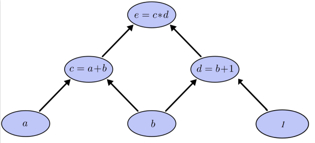
The expression of this graph is not complicated: e = (a+b)*(b+1). Let’s start from the bottom of the graph. The nodes at the lowest level of the graph are called leaves. The leaves of the graph do not accept inputs and only provides a Tensor as output. Actually, a Tensor would not be in a non-leaf node for this reason. The three leaves are variables a and b, and a constant 1.
One level up is two operation nodes. Each one of them represents an addition. Both take two inputs from the nodes below. These middle and higher levels depend on their predecessors, for they could not be computed without the outputs from a, b, or 1. Note that both addition operations are parallel to each other at the same level: Tensorflow does not need to wait on all of them to complete before moving on to the next node.
The final node is a multiplication node. It take c and d as input, forming the expression e = (c)*(d), while c = a+b and d = b+1. Therefore, combining the two expressions, we have the final result of e = (a+b)*(b+1).
That is all for our introduction to basic Tensorflow concepts. We will discuss further advanced features of Tensorflow in later posts. Stay tuned and see you next time!
Works Cited

In this blog, we are going to talk about another optimization algorithm, the simulated annealing. As we mentioned last time, the goal of machine learning algorithms is to minimize the difference between the predicted values of the trained model and the actual values from either surveying or measuring or to find the minimum of the error function. Compared to gradient descent method introduced in the previous blog, simulated annealing algorithm offers a more efficient way to find the global maximum instead of a local one in a certain dataset. Though this method is not complex in nature, it requires some understanding of a field of physics that is not widely known and is a bit abstract.
As its name suggests, simulated annealing algorithm is derived from the annealing process in metallurgy. This process is a controlled heating and then cooling of metal to achieve desired properties, specifically increase the strength of the metal. First, the material is heated up to its melting point and is cast and formed. Heat, at the atomic level, is represented as the kinetic energy of particles. During this stage, all particles have a tremendous amount of kinetic energy and move rather quickly, since the hotter the material is, the greater kinetic energy the particles possess. As the particles roam through space, it is almost impossible to form chemical bonds and therefore the metal loses its physical form and turns into the liquid.

Then the metal starts to be cooled. As the temperature decreases, the kinetic energy also falls. More particles slow down, and permanent bonds start to form between the atoms. Therefore, small freezing “seeds” came into existence and particles around them form crystals upon the seeds. As seeds slowly grow into larger and larger lattices, particles have enough time to fit into the state of minimum energy, giving the whole piece of metal a more steady structure and minimizing inner tension inside the metal. The cooling process is carefully adjusted so that every atom could end up with the least possible energy. If the process is run too quickly, the result would not be desired.

In simulated annealing, the same method applies. Instead of working with real metal, we treat the problem like an atomic thermodynamic system, “crystallizing” the coefficients of our error function into their lowest “energy” state. A typical simulated annealing includes a number of consecutive jumps across the plot of our error function. The amplitude of each jump is determined by the current temperature of the system. The following is an example of a simulated annealing:

The horizontal axis is the possibility of different coefficients in our error function and the vertical axis is the fitness of our model. In other words, the bigger the value in the graph, the better the coefficients fits the data, and the lower the error.
We start at point 1, which is completely chosen at will. We made a random jump towards point 2. Note that with a high system temperature, such large-scaled jumps are allowed, though it is really likely to end up with a worse landing point than the starting. Now we continue the jump to point 3, which is actually worse than point 2. No worries, “it’s gonna get worse before it gets better”, as the old saying goes. When we accumulate more jumps, the temperature of the system decreases, limiting the amplitude of the jumps. After numerous jumps, we could finally reach point 9, which is the global maximum and is where we end the algorithm as the temperature reaches 0.
Simulated Annealing offers a unique interpretation of a physical model and brings it into the optimization process. The randomness included in the algorithm actually gives it a shorter solving time compared to other optimization processes, marking it with distinctive qualities.
We will continue to explore Tensorflow, the programming package that allows us to build our own artificial intelligence model, in my next post. See you very soon!
Works Cited
“Simulated Annealing, a brief introduction.” I Eat Bugs For Breakfast, 14 Mar. 2012, ieatbugsforbreakfast.wordpress.com/2011/10/14/simulated-annealing-a-brief-introduction/.
